You can find the examples detailed on this page in the examples/ directory of SCOOP.
Please check the API Reference for any implentation detail of the proposed functions.
¶A Monte-Carlo method to
calculate using SCOOP to parallelize its computation is found in
examples/piCalc.py.
You should familiarize yourself with
Monte-Carlo methods before
going forth with this example.
First, we need to import the needed functions as such:
1 2 3 | from math import hypot
from random import random
from scoop import futures
|
The Monte-Carlo method is
then defined. It spawns two pseudo-random numbers that are fed to the
hypot function which
calculates the hypotenuse of its parameters.
This step computes the
Pythagorean equation
( ) of the given parameters to find the distance from the
origin (0,0) to the randomly placed point (which X and Y values were generated
from the two pseudo-random values).
Then, the result is compared to one to evaluate if this point is inside or
outside the unit disk.
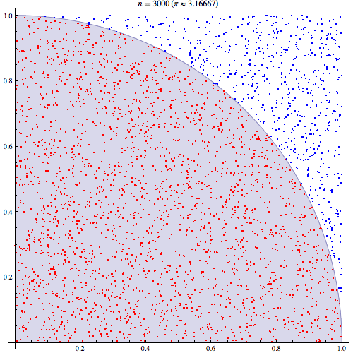
If it is inside (have a distance from the origin lesser than one), a value of
one is produced (red dots in the figure), otherwise the value is zero (blue dots
in the figure).
The experiment is repeated tries number of times with new random values.
) of the given parameters to find the distance from the
origin (0,0) to the randomly placed point (which X and Y values were generated
from the two pseudo-random values).
Then, the result is compared to one to evaluate if this point is inside or
outside the unit disk.
If it is inside (have a distance from the origin lesser than one), a value of
one is produced (red dots in the figure), otherwise the value is zero (blue dots
in the figure).
The experiment is repeated tries number of times with new random values.
The function returns the number times a pseudo-randomly generated point fell inside the unit disk for a given number of tries.
1 2 | def test(tries):
return sum(hypot(random(), random()) < 1 for i in range(tries))
|
One way to obtain a more precise result with a
Monte-Carlo method is to
perform the method multiple times. The following function executes repeatedly
the previous function to gain more precision.
These calls are handled by SCOOP using it’s map()
function.
The results, that is the number of times a random distribution over a 1x1
square hits the unit disk over a
given number of tries, are then summed and divided by the total of tries.
Since we only covered the upper right quadrant of the
unit disk because both parameters
are positive in a cartesian map, the result must be multiplied by 4 to get the
relation between area and circumference, namely
.
1 2 3 | def calcPi(nbFutures, tries):
expr = futures.map(test, [tries] * nbFutures)
return 4. * sum(expr) / float(nbFutures * tries)
|
As stated above, you must wrap your code with a test for the __main__ name. You can now run your code using the command python -m scoop.
1 2 | if __name__ == "__main__":
print("pi = {}".format(calcPi(3000, 5000)))
|
The examples/fullTree.py example holds a pretty good wrap-up of available functionnalities. It notably shows that SCOOP is capable of handling twisted and complex hierarchical requirements.
Getting acquainted with the previous examples is fairly enough to use SCOOP, no need to dive into this complicated example.